
What is Machine Learning:
Machine learning (ML) is an application of artificial intelligence (AI) that provides systems the ability to automatically learn and improve from experience without being explicitly programmed. Machine learning focuses on the development of computer programs that can access data and use it learn for themselves.
Machine learning is a category of algorithm that allows software applications to become more accurate in predicting outcomes without being explicitly programmed. The basic premise of machine learning is to build algorithms that can receive input data and use statistical analysis to predict an output while updating outputs as new data becomes available.
What I'm going to cover in this blog?
I am providing a high level understanding about various machine learning algorithms along with Python & R codes to run them. I have deliberately skipped the statistics behind these techniques, as you don’t need to understand them at the start. So, if you are looking for statistical understanding of these algorithms please check this link. But, if you are looking to equip yourself to start building machine learning project, this blog would be a handy for you.Types of Machine Learning Algorithms
1. Supervised Learning
This algorithm consist of a target / outcome variable (or dependent variable) which is to be predicted from a given set of predictors (independent variables). Using these set of variables, we generate a function that map inputs to desired outputs. The training process continues until the model achieves a desired level of accuracy on the training data. Examples of Supervised Learning: Regression, Decision Tree, Random Forest, KNN, Logistic Regression etc.
2. Unsupervised Learning
In this algorithm, we do not have any target or outcome variable to predict / estimate. It is used for clustering population in different groups, which is widely used for segmenting customers in different groups for specific intervention. Examples of Unsupervised Learning: Apriori algorithm, K-means.
3. Reinforcement Learning:
Using this algorithm, the machine is trained to make specific decisions. It works this way: the machine is exposed to an environment where it trains itself continually using trial and error. This machine learns from past experience and tries to capture the best possible knowledge to make accurate business decisions. Example of Reinforcement Learning: Markov Decision Process


List of Common Machine Learning Algorithms
Here is the list of commonly used machine learning algorithms. These algorithms can be applied to almost any data problem:

1. Regression:
1.1. Linear Regression
As the name indicates this already, linear regression is well known to be an approach for modeling the relationship that lies in between a dependent variable ‘y’ and another or more independent variables that are denoted as ‘x’ and expressed in a linear form. The word Linear indicates that the dependent variable is directly proportional to the independent variables. There are other things that are to be kept in mind.
It has to be constant as if x is increased/decreased then Y also changes linearly. Mathematically the relationship is based and expressed in the simplest form as: This is
Y = aX + b
Here A and B are considered to be the constant factors. The goal hidden behind the Supervised learning using linear regression is to find the exact value of the Constants ‘A’ and ‘B’ with the help of the data sets. Then these values, i.e. the value of the Constants will be helpful in predicting the values of ‘y’ in the future for any values of ‘x’. Now, the cases where there is a single and independent variable it is termed as simple linear regression, while if there is the chance of more than one independent variable, then this process is called multiple linear regression.
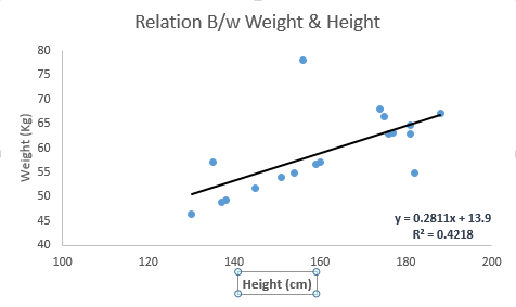
The best way to understand linear regression is to relive this experience of childhood. Let us say, you ask a child in fifth grade to arrange people in his class by increasing order of weight, without asking them their weights! What do you think the child will do? He / she would likely look (visually analyze) at the height and build of people and arrange them using a combination of these visible parameters. This is linear regression in real life! The child has actually figured out that height and build would be correlated to the weight by a relationship, which looks like the equation above.
In this equation:
- Y – Dependent Variable
- a – Slope
- X – Independent variable
- b – Intercept
These coefficients a and b are derived based on minimizing the sum of squared difference of distance between data points and regression line.
Look at the below example. Here we have identified the best fit line having linear equation y=0.2811x+13.9. Now using this equation, we can find the weight, knowing the height of a person.
Linear Regression is of mainly two types: Simple Linear Regression and Multiple Linear Regression. Simple Linear Regression is characterized by one independent variable. And, Multiple Linear Regression(as the name suggests) is characterized by multiple (more than 1) independent variables. While finding best fit line, you can fit a polynomial or curvilinear regression. And these are known as polynomial or curvilinear regression.
Python Code
#Import Library
#Import other necessary libraries like pandas, numpy...
from sklearn import linear_model
#Load Train and Test datasets
#Identify feature and response variable(s) and values must be numeric and numpy arrays
x_train=input_variables_values_training_datasets
y_train=target_variables_values_training_datasets
x_test=input_variables_values_test_datasets
# Create linear regression object
linear = linear_model.LinearRegression()
# Train the model using the training sets and check score
linear.fit(x_train, y_train)
linear.score(x_train, y_train)
#Equation coefficient and Intercept
print('Coefficient: \n', linear.coef_)
print('Intercept: \n', linear.intercept_)
#Predict Output
predicted= linear.predict(x_test)
R Code
#Load Train and Test datasets
#Identify feature and response variable(s) and values must be numeric and numpy arrays
x_train <- input_variables_values_training_datasets
y_train <- target_variables_values_training_datasets
x_test <- input_variables_values_test_datasets
x <- cbind(x_train,y_train)
# Train the model using the training sets and check score
linear <- lm(y_train ~ ., data = x)
summary(linear)
#Predict Output
predicted= predict(linear,x_test)
1.2. Decision Tree
This is one of my favorite algorithm and I use it quite frequently. It is a type of supervised learning algorithm that is mostly used for classification problems. Surprisingly, it works for both categorical and continuous dependent variables. In this algorithm, we split the population into two or more homogeneous sets. This is done based on most significant attributes/ independent variables to make as distinct groups as possible. For more details, you can read: Decision Tree Simplified.
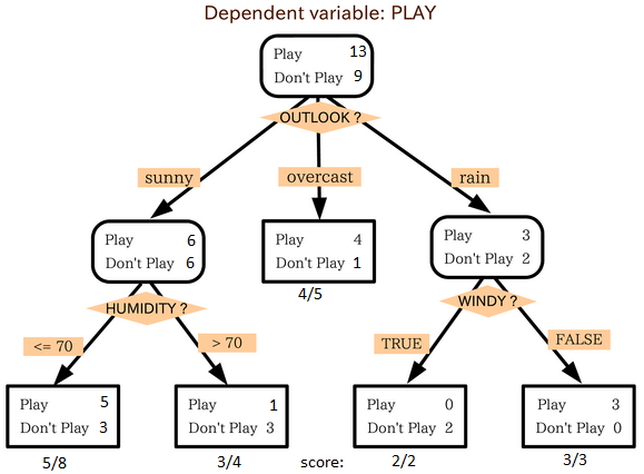 source: statsexchange
In the image above, you can see that population is classified into four different groups based on multiple attributes to identify ‘if they will play or not’. To split the population into different heterogeneous groups, it uses various techniques like Gini, Information Gain, Chi-square, entropy.
The best way to understand how decision tree works, is to play Jezzball – a classic game from Microsoft (image below). Essentially, you have a room with moving walls and you need to create walls such that maximum area gets cleared off with out the balls.
source: statsexchange
In the image above, you can see that population is classified into four different groups based on multiple attributes to identify ‘if they will play or not’. To split the population into different heterogeneous groups, it uses various techniques like Gini, Information Gain, Chi-square, entropy.
The best way to understand how decision tree works, is to play Jezzball – a classic game from Microsoft (image below). Essentially, you have a room with moving walls and you need to create walls such that maximum area gets cleared off with out the balls.
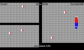 So, every time you split the room with a wall, you are trying to create 2 different populations with in the same room. Decision trees work in very similar fashion by dividing a population in as different groups as possible.
This is one of my favorite algorithm and I use it quite frequently. It is a type of supervised learning algorithm that is mostly used for classification problems. Surprisingly, it works for both categorical and continuous dependent variables. In this algorithm, we split the population into two or more homogeneous sets. This is done based on most significant attributes/ independent variables to make as distinct groups as possible. For more details, you can read: Decision Tree Simplified.
Python Code
#Import Library
#Import other necessary libraries like pandas, numpy...
from sklearn import tree
#Assumed you have, X (predictor) and Y (target) for training data set and x_test(predictor) of test_dataset
# Create tree object
model = tree.DecisionTreeClassifier(criterion='gini') # for classification, here you can change the algorithm as gini or entropy (information gain) by default it is gini
# model = tree.DecisionTreeRegressor() for regression
# Train the model using the training sets and check score
model.fit(X, y)
model.score(X, y)
#Predict Output
predicted= model.predict(x_test)
R Code
library(rpart)
x <- cbind(x_train,y_train)
# grow tree
fit <- rpart(y_train ~ ., data = x,method="class")
summary(fit)
#Predict Output
predicted= predict(fit,x_test)
1.3. Random Forest
Random Forest is a trademark term for an ensemble of decision trees. In Random Forest, we’ve collection of decision trees (so known as “Forest”). To classify a new object based on attributes, each tree gives a classification and we say the tree “votes” for that class. The forest chooses the classification having the most votes (over all the trees in the forest).
Each tree is planted & grown as follows:
- If the number of cases in the training set is N, then sample of N cases is taken at random but with replacement. This sample will be the training set for growing the tree.
- If there are M input variables, a number m<<M is specified such that at each node, m variables are selected at random out of the M and the best split on these m is used to split the node. The value of m is held constant during the forest growing.
- Each tree is grown to the largest extent possible. There is no pruning.
For more details on this algorithm, comparing with decision tree and tuning model parameters, I would suggest you to read these articles:
-
-
-
-
Python
#Import Library
from sklearn.ensemble import RandomForestClassifier
#Assumed you have, X (predictor) and Y (target) for training data set and x_test(predictor) of test_dataset
# Create Random Forest object
model= RandomForestClassifier()
# Train the model using the training sets and check score
model.fit(X, y)
#Predict Output
predicted= model.predict(x_test)
R Code
library(randomForest)
x <- cbind(x_train,y_train)
# Fitting model
fit <- randomForest(Species ~ ., x,ntree=500)
summary(fit)
#Predict Output
predicted= predict(fit,x_test)
Random Forest is a trademark term for an ensemble of decision trees. In Random Forest, we’ve collection of decision trees (so known as “Forest”). To classify a new object based on attributes, each tree gives a classification and we say the tree “votes” for that class. The forest chooses the classification having the most votes (over all the trees in the forest).
2. Classification:
2.1. Logistic Regression
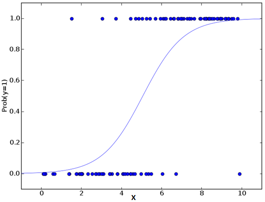
Don’t get confused by its name! It is a classification not a regression algorithm. It is used to estimate discrete values ( Binary values like 0/1, yes/no, true/false ) based on given set of independent variable(s). In simple words, it predicts the probability of occurrence of an event by fitting data to a logit function. Hence, it is also known as logit regression. Since, it predicts the probability, its output values lies between 0 and 1 (as expected).
Again, let us try and understand this through a simple example.
Let’s say your friend gives you a puzzle to solve. There are only 2 outcome scenarios – either you solve it or you don’t. Now imagine, that you are being given wide range of puzzles / quizzes in an attempt to understand which subjects you are good at. The outcome to this study would be something like this – if you are given a trignometry based tenth grade problem, you are 70% likely to solve it. On the other hand, if it is grade fifth history question, the probability of getting an answer is only 30%. This is what Logistic Regression provides you.
Coming to the math, the log odds of the outcome is modeled as a linear combination of the predictor variables.
odds= p/ (1-p) = probability of event occurrence / probability of not event occurrence
ln(odds) = ln(p/(1-p))
logit(p) = ln(p/(1-p)) = b0+b1X1+b2X2+b3X3....+bkXk
Above, p is the probability of presence of the characteristic of interest. It chooses parameters that maximize the likelihood of observing the sample values rather than that minimize the sum of squared errors (like in ordinary regression).
Now, you may ask, why take a log? For the sake of simplicity, let’s just say that this is one of the best mathematical way to replicate a step function. I can go in more details, but that will beat the purpose of this article.
 Python Code
#Import Library
from sklearn.linear_model import LogisticRegression
#Assumed you have, X (predictor) and Y (target) for training data set and x_test(predictor) of test_dataset
# Create logistic regression object
model = LogisticRegression()
# Train the model using the training sets and check score
model.fit(X, y)
model.score(X, y)
#Equation coefficient and Intercept
print('Coefficient: \n', model.coef_)
print('Intercept: \n', model.intercept_)
#Predict Output
predicted= model.predict(x_test)
R Code
x <- cbind(x_train,y_train)
# Train the model using the training sets and check score
logistic <- glm(y_train ~ ., data = x,family='binomial')
summary(logistic)
#Predict Output
predicted= predict(logistic,x_test)
Don’t get confused by its name! It is a classification not a regression algorithm. It is used to estimate discrete values ( Binary values like 0/1, yes/no, true/false ) based on given set of independent variable(s). In simple words, it predicts the probability of occurrence of an event by fitting data to a logit function. Hence, it is also known as logit regression. Since, it predicts the probability, its output values lies between 0 and 1 (as expected).
Python Code
2.2 kNN (k- Nearest Neighbors)
2.2 kNN (k- Nearest Neighbors)
It can be used for both classification and regression problems. However, it is more widely used in classification problems in the industry. K nearest neighbors is a simple algorithm that stores all available cases and classifies new cases by a majority vote of its k neighbors. The case being assigned to the class is most common amongst its K nearest neighbors measured by a distance function.
These distance functions can be Euclidean, Manhattan, Minkowski and Hamming distance. First three functions are used for continuous function and fourth one (Hamming) for categorical variables. If K = 1, then the case is simply assigned to the class of its nearest neighbor. At times, choosing K turns out to be a challenge while performing kNN modeling.
 KNN can easily be mapped to our real lives. If you want to learn about a person, of whom you have no information, you might like to find out about his close friends and the circles he moves in and gain access to his/her information!
Things to consider before selecting kNN:
KNN can easily be mapped to our real lives. If you want to learn about a person, of whom you have no information, you might like to find out about his close friends and the circles he moves in and gain access to his/her information!
Things to consider before selecting kNN:
- KNN is computationally expensive
- Variables should be normalized else higher range variables can bias it
- Works on pre-processing stage more before going for kNN like outlier, noise removal
Python Code
#Import Library
from sklearn.neighbors import KNeighborsClassifier
#Assumed you have, X (predictor) and Y (target) for training data set and x_test(predictor) of test_dataset
# Create KNeighbors classifier object model
KNeighborsClassifier(n_neighbors=6) # default value for n_neighbors is 5
# Train the model using the training sets and check score
model.fit(X, y)
#Predict Output
predicted= model.predict(x_test)
R Code
library(knn)
x <- cbind(x_train,y_train)
# Fitting model
fit <-knn(y_train ~ ., data = x,k=5)
summary(fit)
#Predict Output
predicted= predict(fit,x_test)
2.3. SVM (Support Vector Machine)
It is a classification method. In this algorithm, we plot each data item as a point in n-dimensional space (where n is number of features you have) with the value of each feature being the value of a particular coordinate.
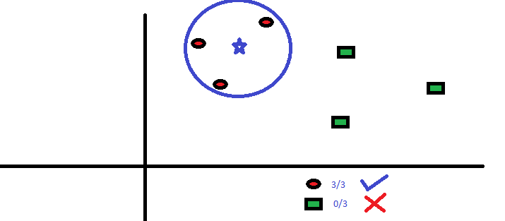
For example, if we only had two features like Height and Hair length of an individual, we’d first plot these two variables in two dimensional space where each point has two co-ordinates (these co-ordinates are known as Support Vectors)
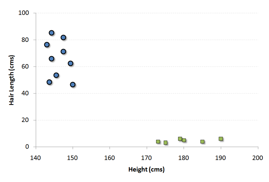 Now, we will find some line that splits the data between the two differently classified groups of data. This will be the line such that the distances from the closest point in each of the two groups will be farthest away.
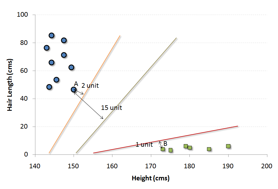
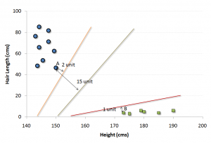 In the example shown above, the line which splits the data into two differently classified groups is the black line, since the two closest points are the farthest apart from the line. This line is our classifier. Then, depending on where the testing data lands on either side of the line, that’s what class we can classify the new data as.
Think of this algorithm as playing JezzBall in n-dimensional space. The tweaks in the game are:
In the example shown above, the line which splits the data into two differently classified groups is the black line, since the two closest points are the farthest apart from the line. This line is our classifier. Then, depending on where the testing data lands on either side of the line, that’s what class we can classify the new data as.
Think of this algorithm as playing JezzBall in n-dimensional space. The tweaks in the game are:
- You can draw lines / planes at any angles (rather than just horizontal or vertical as in classic game)
- The objective of the game is to segregate balls of different colors in different rooms.
- And the balls are not moving.
It is a classification method. In this algorithm, we plot each data item as a point in n-dimensional space (where n is number of features you have) with the value of each feature being the value of a particular coordinate.
Python Code
#Import Library
from sklearn import svm
#Assumed you have, X (predictor) and Y (target) for training data set and x_test(predictor) of test_dataset
# Create SVM classification object
model = svm.svc() # there is various option associated with it, this is simple for classification. You can refer link, for mo# re detail.
# Train the model using the training sets and check score
model.fit(X, y)
model.score(X, y)
#Predict Output
predicted= model.predict(x_test)
R Code
library(e1071)
x <- cbind(x_train,y_train)
# Fitting model
fit <-svm(y_train ~ ., data = x)
summary(fit)
#Predict Output
predicted= predict(fit,x_test)
3.4. Naive Bayes
3.4. Naive Bayes
It is a classification technique based on Bayes’ theorem with an assumption of independence between predictors. In simple terms, a Naive Bayes classifier assumes that the presence of a particular feature in a class is unrelated to the presence of any other feature. For example, a fruit may be considered to be an apple if it is red, round, and about 3 inches in diameter. Even if these features depend on each other or upon the existence of the other features, a naive Bayes classifier would consider all of these properties to independently contribute to the probability that this fruit is an apple.
Naive Bayesian model is easy to build and particularly useful for very large data sets. Along with simplicity, Naive Bayes is known to outperform even highly sophisticated classification methods.
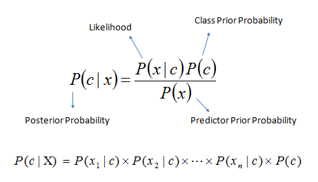
Bayes theorem provides a way of calculating posterior probability P(c|x) from P(c), P(x) and P(x|c). Look at the equation below:
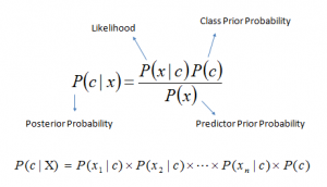 Here,
Here,
- P(c|x) is the posterior probability of class (target) given predictor (attribute).
- P(c) is the prior probability of class.
- P(x|c) is the likelihood which is the probability of predictor given class.
- P(x) is the prior probability of predictor.
Example: Let’s understand it using an example. Below I have a training data set of weather and corresponding target variable ‘Play’. Now, we need to classify whether players will play or not based on weather condition. Let’s follow the below steps to perform it.
Step 1: Convert the data set to frequency table
Step 2: Create Likelihood table by finding the probabilities like Overcast probability = 0.29 and probability of playing is 0.64.
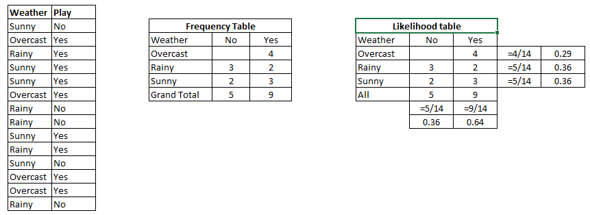 Step 3: Now, use Naive Bayesian equation to calculate the posterior probability for each class. The class with the highest posterior probability is the outcome of prediction.
Problem: Players will pay if weather is sunny, is this statement is correct?
We can solve it using above discussed method, so P(Yes | Sunny) = P( Sunny | Yes) * P(Yes) / P (Sunny)
Here we have P (Sunny |Yes) = 3/9 = 0.33, P(Sunny) = 5/14 = 0.36, P( Yes)= 9/14 = 0.64
Now, P (Yes | Sunny) = 0.33 * 0.64 / 0.36 = 0.60, which has higher probability.
Naive Bayes uses a similar method to predict the probability of different class based on various attributes. This algorithm is mostly used in text classification and with problems having multiple classes.
Step 3: Now, use Naive Bayesian equation to calculate the posterior probability for each class. The class with the highest posterior probability is the outcome of prediction.
Problem: Players will pay if weather is sunny, is this statement is correct?
We can solve it using above discussed method, so P(Yes | Sunny) = P( Sunny | Yes) * P(Yes) / P (Sunny)
Here we have P (Sunny |Yes) = 3/9 = 0.33, P(Sunny) = 5/14 = 0.36, P( Yes)= 9/14 = 0.64
Now, P (Yes | Sunny) = 0.33 * 0.64 / 0.36 = 0.60, which has higher probability.
Naive Bayes uses a similar method to predict the probability of different class based on various attributes. This algorithm is mostly used in text classification and with problems having multiple classes.
It is a classification technique based on Bayes’ theorem with an assumption of independence between predictors. In simple terms, a Naive Bayes classifier assumes that the presence of a particular feature in a class is unrelated to the presence of any other feature. For example, a fruit may be considered to be an apple if it is red, round, and about 3 inches in diameter. Even if these features depend on each other or upon the existence of the other features, a naive Bayes classifier would consider all of these properties to independently contribute to the probability that this fruit is an apple.
Python Code
#Import Library
from sklearn.naive_bayes import GaussianNB
#Assumed you have, X (predictor) and Y (target) for training data set and x_test(predictor) of test_dataset
# Create SVM classification object model = GaussianNB() # there is other distribution for multinomial classes like Bernoulli Naive Bayes, Refer link
# Train the model using the training sets and check score
model.fit(X, y)
#Predict Output
predicted= model.predict(x_test)
R Code
library(e1071)
x <- cbind(x_train,y_train)
# Fitting model
fit <-naiveBayes(y_train ~ ., data = x)
summary(fit)
#Predict Output
predicted= predict(fit,x_test)
4.Clustering:
4.Clustering:
4.1. K-Means
It is a type of unsupervised algorithm which solves the clustering problem. Its procedure follows a simple and easy way to classify a given data set through a certain number of clusters (assume k clusters). Data points inside a cluster are homogeneous and heterogeneous to peer groups.
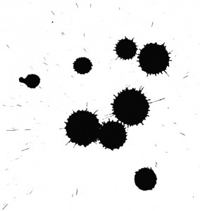
Remember figuring out shapes from ink blots? k means is somewhat similar this activity. You look at the shape and spread to decipher how many different clusters / population are present!
 How K-means forms cluster:
- K-means picks k number of points for each cluster known as centroids.
- Each data point forms a cluster with the closest centroids i.e. k clusters.
- Finds the centroid of each cluster based on existing cluster members. Here we have new centroids.
- As we have new centroids, repeat step 2 and 3. Find the closest distance for each data point from new centroids and get associated with new k-clusters. Repeat this process until convergence occurs i.e. centroids does not change.
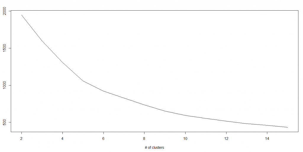
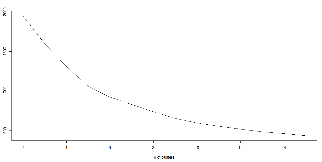
How to determine value of K:
In K-means, we have clusters and each cluster has its own centroid. Sum of square of difference between centroid and the data points within a cluster constitutes within sum of square value for that cluster. Also, when the sum of square values for all the clusters are added, it becomes total within sum of square value for the cluster solution.
We know that as the number of cluster increases, this value keeps on decreasing but if you plot the result you may see that the sum of squared distance decreases sharply up to some value of k, and then much more slowly after that. Here, we can find the optimum number of cluster.
Python Code
#Import Library
from sklearn.cluster import KMeans
#Assumed you have, X (attributes) for training data set and x_test(attributes) of test_dataset
# Create KNeighbors classifier object model
k_means = KMeans(n_clusters=3, random_state=0)
# Train the model using the training sets and check score
model.fit(X)
#Predict Output
predicted= model.predict(x_test)
R Code
library(cluster)
fit <- kmeans(X, 3) # 5 cluster solution
4.2. Hierarchical Clustering
Hierarchical clustering is an alternative approach to k-means clustering for identifying groups in the dataset and does not require to pre-specify the number of clusters to generate.
It refers to a set of clustering algorithms that build tree-like clusters by successively splitting or merging them. This hierarchical structure is represented using a tree.
Hierarchical clustering methods use a distance similarity measure to combine or split clusters. The recursive process continues until there is only one cluster left or we cannot split more clusters. We can use a dendrogram to represent the hierarchy of clusters.
Dendrogram
A dendrogram is a tree-like structure frequently used to illustrate the arrangement of the clusters produced by hierarchical clustering.
Hierarchical classifications produced by either
1. Agglomerative
2. Divisive
The agglomerative or divisive route may be represented by a two-dimensional diagram known as a dendrogram, which illustrates the fusions or divisions made at each stage of the analysis.Agglomerative clustering usually yields a higher number of clusters, with fewer leaf nodes in the cluster.
In a hierarchical classification, the data are not partitioned into a particular number of classes or clusters at a single step. Instead, the classification consists of a series of partitions, which may run from a single cluster containing all individuals to n clusters each containing a single individual.
Hierarchical clustering algorithms can be either bottom-up or top-down.

Hierarchical clustering agglomerative and divisive methods
Agglomerative clustering
Agglomerative clustering is Bottom-up technique start by considering each data point as its own cluster and merging them together into larger groups from the bottom up into a single giant cluster.
Divisive clustering
Divisive clustering is the opposite, it starts with one cluster, which is then divided in two as a function of the similarities or distances in the data. These new clusters are then divided, and so on until each case is a cluster.
Python Code
# Using the dendrogram to find the optimal number of clusters
import scipy.cluster.hierarchy as sch
dendrogram = sch.dendrogram(sch.linkage(X, method = 'ward'))
plt.title('Dendrogram')
plt.xlabel('Customers')
plt.ylabel('Euclidean distances')
plt.show()

# Fitting Hierarchical Clustering to the dataset
from sklearn.cluster import AgglomerativeClustering
hc = AgglomerativeClustering(n_clusters = 5, affinity = 'euclidean', linkage = 'ward')
y_hc = hc.fit_predict(X)

# Visualising the clusters
plt.scatter(X[y_hc == 0, 0], X[y_hc == 0, 1], s = 100, c = 'red', label = 'Cluster 1')
plt.scatter(X[y_hc == 1, 0], X[y_hc == 1, 1], s = 100, c = 'blue', label = 'Cluster 2')
plt.scatter(X[y_hc == 2, 0], X[y_hc == 2, 1], s = 100, c = 'green', label = 'Cluster 3')
plt.scatter(X[y_hc == 3, 0], X[y_hc == 3, 1], s = 100, c = 'cyan', label = 'Cluster 4')
plt.scatter(X[y_hc == 4, 0], X[y_hc == 4, 1], s = 100, c = 'magenta', label = 'Cluster 5')
plt.title('Clusters of customers')
plt.xlabel('Annual Income (k$)')
plt.ylabel('Spending Score (1-100)')
plt.legend()
plt.show()
R Code
# Hierarchical Clustering
# test_set = scale(test_set)
# Using the dendrogram to find the optimal number of clusters
dendrogram = hclust(d = dist(dataset, method = 'euclidean'), method = 'ward.D')
plot(dendrogram,
     main = paste('Dendrogram'),
     xlab = 'Customers',
     ylab = 'Euclidean distances')
# Fitting Hierarchical Clustering to the dataset
hc = hclust(d = dist(dataset, method = 'euclidean'), method = 'ward.D')
y_hc = cutree(hc, 5)
# Visualising the clusters
library(cluster)
clusplot(dataset,
         y_hc,
         lines = 0,
         shade = TRUE,
         color = TRUE,
         labels= 2,
         plotchar = FALSE,
         span = TRUE,
         main = paste('Clusters of customers'),
         xlab = 'Annual Income',
         ylab = 'Spending Score')
5. Association Rule Learning:
# Hierarchical Clustering
# test_set = scale(test_set)
# Using the dendrogram to find the optimal number of clusters
dendrogram = hclust(d = dist(dataset, method = 'euclidean'), method = 'ward.D')
plot(dendrogram,
main = paste('Dendrogram'),
xlab = 'Customers',
ylab = 'Euclidean distances')
# Fitting Hierarchical Clustering to the dataset
hc = hclust(d = dist(dataset, method = 'euclidean'), method = 'ward.D')
y_hc = cutree(hc, 5)
# Visualising the clusters
library(cluster)
clusplot(dataset,
y_hc,
lines = 0,
shade = TRUE,
color = TRUE,
labels= 2,
plotchar = FALSE,
span = TRUE,
main = paste('Clusters of customers'),
xlab = 'Annual Income',
ylab = 'Spending Score')
5. Association Rule Learning:5.1. Apriori
Apriori uses a breadth-first search strategy to count the support of itemsets and uses a candidate generation function which exploits the downward closure property of support.
Apriori algorithm is a classical algorithm in data mining. It is used for mining frequent itemsets and relevant association rules. It is devised to operate on a database containing a lot of transactions, for instance, items brought by customers in a store.
It is very important for effective Market Basket Analysis and it helps the customers in purchasing their items with more ease which increases the sales of the markets. It has also been used in the field of healthcare for the detection of adverse drug reactions. It produces association rules that indicates what all combinations of medications and patient characteristics lead to ADRs.
Python Code
# Apriori
# Importing the libraries
import numpy as np
import matplotlib.pyplot as plt
import pandas as pd

# Training Apriori on the dataset
from apyori import apriori
rules = apriori(transactions, min_support = 0.003, min_confidence = 0.2, min_lift = 3, min_length = 2)

# Visualising the results
results = list(rules)
R Code
# Apriori

# Training Apriori on the dataset
rules = apriori(data = dataset, parameter = list(support = 0.004, confidence = 0.2))

# Visualising the results
inspect(sort(rules, by = 'lift')[1:10])
5.2. Eclat
Eclat (alt. ECLAT, stands for Equivalence Class Transformation) is a depth-first search algorithm based on set intersection. It is suitable for both sequential as well as parallel execution with locality-enhancing properties
The basic idea for the eclat algorithm is use tidset intersections to compute the support of a candidate itemset avoiding the generation of subsets that does not exist in the prefix tree.
# Eclat
# Data Preprocessing
# install.packages('arules')
library(arules)
dataset = read.csv('Market_Basket_Optimisation.csv')
dataset = read.transactions('Market_Basket_Optimisation.csv', sep = ',', rm.duplicates = TRUE)
summary(dataset)
itemFrequencyPlot(dataset, topN = 10)

# Training Eclat on the dataset
rules = eclat(data = dataset, parameter = list(support = 0.003, minlen = 2))

# Visualising the results
inspect(sort(rules, by = 'support')[1:10])
6. Dimensionality reduction:
In statistics, machine learning, and information theory, dimensionality reduction or dimension reduction is the process of reducing the number of random variables under consideration[1] by obtaining a set of principal variables. It can be divided into feature selection and feature extraction.
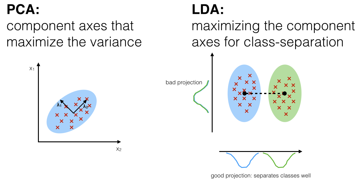
Linear Discriminant Analysis (LDA) is most commonly used as dimensionality reduction technique in the pre-processing step for pattern-classification and machine learning applications. The goal is to project a dataset onto a lower-dimensional space with good class-separability in order avoid overfitting (“curse of dimensionality”) and also reduce computational costs.6.1. Principal Component Analysis (PCA)
Principal component analysis (PCA) is a statistical procedure that uses an orthogonal transformation to convert a set of observations of possibly correlated variables (entities each of which takes on various numerical values) into a set of values of linearly uncorrelated variables called principal components.
In simple terms it's a method of analysis which involves finding the linear combination of a set of variables that has maximum variance and removing its effect, repeating this successively.
Python Code
# PCA
# Importing the libraries
import numpy as np
import matplotlib.pyplot as plt
import pandas as pd

from sklearn.decomposition import PCA
pca = PCA(n_components = 2)
X_train = pca.fit_transform(X_train)
X_test = pca.transform(X_test)
explained_variance = pca.explained_variance_ratio_
R Code
# PCA
# Importing the dataset
dataset = read.csv('Wine.csv')

# Applying PCA
# install.packages('caret')
library(caret)
# install.packages('e1071')
library(e1071)
pca = preProcess(x = training_set[-14], method = 'pca', pcaComp = 2)
training_set = predict(pca, training_set)
training_set = training_set[c(2, 3, 1)]
test_set = predict(pca, test_set)
test_set = test_set[c(2, 3, 1)]
6.2. Linear Discriminant Analysis (LDA)
Below are the 5 general steps for performing a linear discriminant analysis:
- Compute the d-dimensional mean vectors for the different classes from the dataset.
- Compute the scatter matrices (in-between-class and within-class scatter matrix).
- Compute the eigenvectors (ee1,ee2,...,eed) and corresponding eigenvalues (λλ1,λλ2,...,λλd) for the scatter matrices.
- Sort the eigenvectors by decreasing eigenvalues and choose k eigenvectors with the largest eigenvalues to form a d×k dimensional matrix WW (where every column represents an eigenvector).
- Use this d×k eigenvector matrix to transform the samples onto the new subspace. This can be summarized by the matrix multiplication: YY=XX×WW (where XX is a n×d-dimensional matrix representing the n samples, and yy are the transformed n×k-dimensional samples in the new subspace).
A comparison of PCA and LDA:
Python Code
# LDA
# Importing the libraries
import numpy as np
import matplotlib.pyplot as plt
import pandas as pd

# Importing the dataset
dataset = pd.read_csv('Wine.csv')
X = dataset.iloc[:, 0:13].values
y = dataset.iloc[:, 13].values

# Applying LDA
from sklearn.discriminant_analysis import LinearDiscriminantAnalysis as LDA
lda = LDA(n_components = 2)
X_train = lda.fit_transform(X_train, y_train)
X_test = lda.transform(X_test)
R Code
# LDA
# Importing the dataset
dataset = read.csv('Wine.csv')

# Applying LDA
library(MASS)
lda = lda(formula = Customer_Segment ~ ., data = training_set)
training_set = as.data.frame(predict(lda, training_set))
training_set = training_set[c(5, 6, 1)]
test_set = as.data.frame(predict(lda, test_set))

test_set = test_set[c(5, 6, 1)]
test_set = test_set[c(5, 6, 1)]
6. Neural Network
Neural networks are a set of algorithms, modeled loosely after the human brain, that are designed to recognize patterns. They interpret sensory data through a kind of machine perception, labeling or clustering raw input. The patterns they recognize are numerical, contained in vectors, into which all real-world data, be it images, sound, text or time series, must be translated.
Deep learning is the name we use for “stacked neural networks”; that is, networks composed of several layers.
The layers are made of nodes. A node is just a place where computation happens, loosely patterned on a neuron in the human brain, which fires when it encounters sufficient stimuli. A node combines input from the data with a set of coefficients, or weights, that either amplify or dampen that input, thereby assigning significance to inputs for the task the algorithm is trying to learn.
6.1 Artificial Neural networks
An artificial neuron network (ANN) is a computational model based on the structure and functions of biological neural networks. Information that flows through the network affects the structure of the ANN because a neural network changes - or learns, in a sense - based on that input and output.
ANNs are considered nonlinear statistical data modeling tools where the complex relationships between inputs and outputs are modeled or patterns are found.
An ANN has several advantages but one of the most recognized of these is the fact that it can actually learn from observing data sets. In this way, ANN is used as a random function approximation tool. These types of tools help estimate the most cost-effective and ideal methods for arriving at solutions while defining computing functions or distributions. ANN takes data samples rather than entire data sets to arrive at solutions, which saves both time and money. ANNs are considered fairly simple mathematical models to enhance existing data analysis technologies.
ANNs have three layers that are interconnected. The first layer consists of input neurons. Those neurons send data on to the second layer, which in turn sends the output neurons to the third layer.
Training an artificial neural network involves choosing from allowed models for which there are several associated algorithms.
6.2 Convolutional Neural networks
6.2 Convolutional Neural networks
A convolutional neural network (CNN) is a type of artificial neural network used in image recognition and processing that is specifically designed to process pixel data.
CNNs are powerful image processing, artificial intelligence (AI) that use deep learning to perform both generative and descriptive tasks, often using machine vison that
includes image and video recognition, along with recommender systems and natural language processing (NLP).
A neural network is a system of hardware and/or software patterned after the operation of neurons in the human brain. Traditional neural networks are not ideal for image processing and must be fed images in reduced-resolution pieces. CNN have their “neurons” arranged more like those of the frontal lobe, the area responsible for processing visual stimuli in humans and other animals. The layers of neurons are arranged in such a way as to cover the entire visual field avoiding the piecemeal image processing problem of traditional neural networks.
A CNN uses a system much like a multilayer perceptron that has been designed for reduced processing requirements. The layers of a CNN consist of an input layer, an output layer and a hidden layer that includes multiple convolutional layers, pooling layers, fully connected layers and normalization layers. The removal of limitations and increase in efficiency for image processing results in a system that is far more effective, simpler to trains limited for image processing and natural language processing.
6.3 Recurrent Neural Networks
A recurrent neural network (RNN) is a type of artificial neural network commonly used in speech recognition and natural language processing (NLP). RNNs are designed to recognize a data's sequential characteristics and use patterns to predict the next likely scenario.
How recurrent neural networks learn
Artificial neural networks are created with interconnected data processing components that are loosely designed to function like the human brain. They are composed of layers of artificial neurons (network nodes) that have the capability to process input and forward output to other nodes in the network. The nodes are connected by edges or weights that influence a signal's strength and the network's ultimate output.
In some cases, artificial neural networks process information in a single direction from input to output. These "feedforward" neural networks include convolutional neural networks that underpin image recognition systems . RNNs, on the other hand, can be layered to process information in two directions.
Like feedforward neural networks, RNNs can process data from initial input to final output. Unlike feedforward neural networks, RNNs use feedback loops such as Backpropagation Through Time or BPTT throughout the computational process to loop information back into the network. This connects inputs together and is what enables RNNs to process sequential and temporal data.
One drawback to standard RNNs is the vanishing gradient problem, in which performance of the neural network suffers because it can't be trained properly. This happens with deeply layered neural networks, which are used to process complex data.
Standard RNNs that use a gradient-based learning method degrade the bigger and more complex they get. Tuning the parameters effectively at the earliest layers becomes too time consuming and computationally expensive.
One solution to the problem is called Long Short-Term Memory (LSTM) units RNNs built with LSTM units categorize data into short term and long term memory cells . Doing so enables RNNs to figure out what data is important and should be remembered and looped back into the network, and what data can be forgotten.
Very good read! Do you happen to know where Tensorflow and ML.NET stand in this article's context and how they compare to each other?
ReplyDeleteThanks,
James
Looking for Industrial Automation Companies In USA then Mitsubishi is one of the finest companies which provide the best automation services.
ReplyDeleteYou can also visit - https://mitsubishisolutions.com/machine-tool/automation-solutions